Project 2 Final Report

1. Introduction

The motivation behind this project is to build machine learning models that can predict the quality of Portuguese red wine based on physicochemical attributes. Such predictive models can help winemakers and quality control departments take early actions in the wine production process, such as adjusting ingredient concentrations or modifying fermentation strategies, to achieve higher-quality wine. Predicting wine quality can also support better marketing decisions and pricing strategies.

The dataset is suitable for data mining because it consists of multiple continuous variables that influence the outcome. The problem has real-world applications and can yield actionable knowledge in quality assessment and control.

2. Results

Our experiments examined six different classification models on two types of classification problems—binary and multi-class. Each model was evaluated with and without PCA to measure the impact of dimensionality reduction.

2.1 Are Both Classification Problems Equally Predictable?

No. Binary classification was more predictable. It involved separating wines into just two categories, which is inherently simpler and requires less model complexity.

For example:
Random Forest achieved 91.25% (binary) vs. 73.75% (multi-class)

2.2 Are All Models Equally Good?

No. There was a significant difference in model performance.
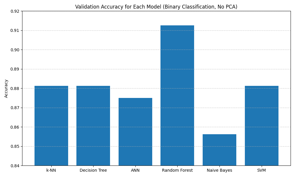
Here we use the Binary Classification task as an example to show the performance of different models.

• Random Forest consistently had the highest validation accuracy across both classification tasks.
• ANN and Decision Tree also performed well, particularly in the binary task.
• Naive Bayes had fast training time and acceptable accuracy, but was limited by its strong independence assumption.
• SVM was moderately effective, but sensitive to hyperparameter tuning and more computationally expensive.

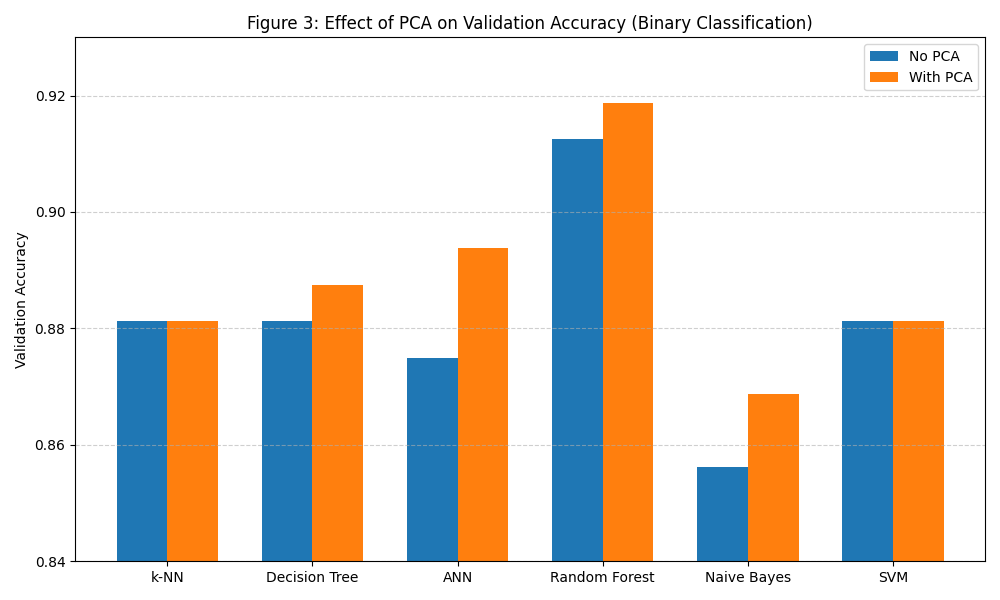
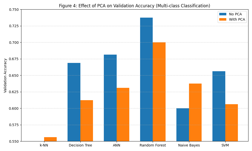
2.3 Did Dimension Reduction Help?

I would say it had a mixed impact.

• In Binary Classification:

  • Most models benefited from PCA. For example, ANN improved from 87.50% to 89.38%, and Random Forest from 91.25% to 91.87%.
  • Naive Bayes also improved, likely due to PCA reducing feature correlations
  • k-NN and SVM showed no performance change, suggesting PCA preserved key data structure.

• In Multi-class Classification:
  The effect of PCA was more mixed.

  • It helped Naive Bayes again from 60.00% to 63.75%. - However, it hurt ANN and SVM, which rely on high-dimensional feature spaces, also Decision Tree, which is sensitive to feature interactions, and Random Forest, which might because of the degradation of classification boundaries.
    
    

2.4 Recommendations

1. For winemakers and quality control experts, whose goal is to detect wine quality as early and accurately as possible during production, Random Forest without PCA is ideal.

2. For marketing and product positioning teams, who may want to segment wines into broad quality levels (low, medium, high), a Naive Bayes classifier with PCA offers fast classification and also acceptable accuracy.

3. For real-time system developers, such as mobile wine review apps, Decision Tree or Naive Bayes with PCA is recommended due to their minimal computational requirements and quick predictions, an Effcient-Cost Tradeoff.

3. Methods

3.1 Dataset and Preprocessing

• Dataset: UCI red wine dataset with 1599 samples
• Features: 11 continuous physicochemical attributes including acidity, sugar content, sulfates, pH, and alcohol content.
• Target: Quality score (0–10), converted to classification labels for binary and multi-class prediction

Preprocessing Steps:

1. Missing value check (none found)
2. Feature scaling (standardization)
3. Label transformation based on defined thresholds

3.2 Classification Problem Definitions

• Binary:

  • Label 0 for quality < 7 (low quality)
  • Label 1 for quality ≥ 7 (high quality)

• Multi-class:

  • Label 0 for quality ≤ 5 (low quality)
  • Label 1 for quality = 6 (medium quality)
  • Label 2 for quality ≥ 7 (high quality)

Rationale: Quality = 6 is the mode of the dataset and forms a logical 'middle class' separating high and low categories.

3.3 Dimension Reduction Method - PCA

Principal Component Analysis (PCA) is an unsupervised linear projection method.
It transforms the original feature space to a set of orthogonal axes (principal components) ordered by variance explained.

We have chosen PCA because of the following reasons:

1. Our dataset contains only continuous, numeric variables, which is ideal for PCA.
2. PCA significantly reduced the dimensionality (from 11 to 5 features) while preserving over 95% of the total variance.
3. It helped speed up training time for all models.

3.4 Hyperparameter Tuning Summary

We used 5-fold cross-validation to select the best hyperparameter values for each model.
For each classification task, we trained each model using different hyperparameter values, and computed the average validation accuracy across the 5 folds.
The value that yielded the highest accuracy was selected for final training and testing.

Model	Hyperparameter	Values Tested	Best Value (Binary)	Best Value (Multi)
k-NN	k	[3, 5, 7, 9, 11]	3	3
Decision Tree	max_depth	[3, 5, 7, 9, 11]	5	9
ANN	hidden layer size	[(50,), (100,), (50, 50)]	(50,)	(50, 50)
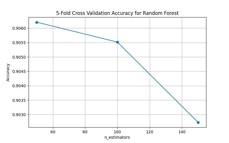
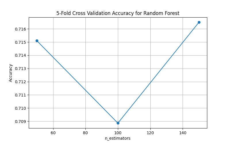
Random Forest	n_estimators	[50, 100, 150]	50	150
Naive Bayes	var_smoothing	[1e-09, 1e-08, 1e-07]	1e-09	1e-09
SVM	C	[0.1, 1, 10]	0.1	10

We chose these hyperparameters carefully:

• For k-NN, smaller values of k helped the model capture more local decision boundaries.
• For Decision Tree, shallower depths helped prevent overfitting, while deeper trees were needed in the multi-class setting to capture more nuanced splits.
• For ANN, it performed best with moderate complexity of the hidden layer size - binary classification favored a single layer of (50,); while multi-class needed deeper structure (50, 50).
• For Random Forest, 50 estimators in binary performed best; the more complex multi-class setting benefited from using 150 trees.
• For Naive Bayes, it benefited from minimal smoothing, suggesting relatively stable likelihood estimates across features.
• For SVM, in the binary classification task, the best penalty C value was 0.1, encouraging a wider margin and better generalization; while SVM required a stronger penalty (C = 10) in the multi-class setting to better separate class boundaries.