Artificial Neural Network
Intro
Basic Structure
- Input nodes: Predictor / Variable values
- Edges: for incoming value , outgoing value is
- Hidden layer nodes: Sum up incoming values term (指 ). Then apply
activation functionto the transformed sum value. - Output nodes: may have additional function before final prediction.
-
Neurons(神经元) = nodes
-
Perception(感知器) = single node binary classifier (Only Input and Output layer)
-
Architecture / Topology: number and organization of nodes, layers, connectors
-
Forward Propagation: Input → Output, applying weights, biases, activation functions
-
Backward Propagation: ← Error (pushed back), adjusting parameters
Activation Function
- ReLU:
- Leaky ReLU: ,
- Sigmoid:
- Tanh:
Calculation
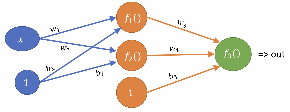
以上:
f(1) = w_1 _ x + b_1
f(2) = w_2 _ x + b_2
f(3) = w_3 _ f(1) + w_4 _ f(2) + b_3
Why multi output nodes?
多分类问题,一个node对应一个预测类别。
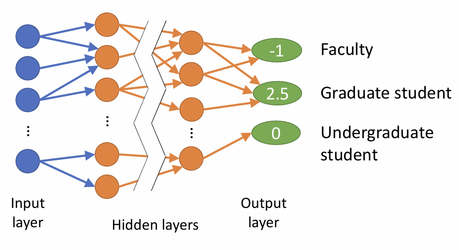
从这个例子看,多个输入特征(Age, Salary...) => 多个输出类别
显然不能作为最后的概率,所以加个激活函数,比如Softmax, 将原始得分转换为概率分布:
所以最终的概率分布为:
而这只是其中一个样本:
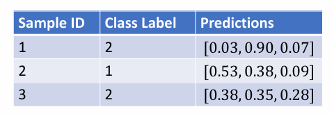
对于所有结果,再用Cross-Entropy Loss计算损失:
再拿它去传回给模型,调整参数。
Wide vs. Deep
理论上,一个足够wide的网络可以拟合任何函数
不过实际上,deep > wide:
- wide 只是memorize,而不是generalize,也就是说它并不能很好地泛化、学习模式
- 神经元随任务复杂程度增加,指数级增长
- deep网络可以自动学习抽象特征
- 小的隐藏层强制网络进行特征抽象 (Feature Abstraction)
- 现实世界的复杂任务本身也通常具有层级结构 (Hierarchical Structure), eg. 图像识别(像素->边缘->形状->物体)
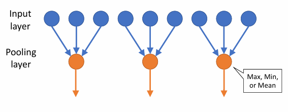
降维 (Dimensionality Reduction) & 压缩 (Compression)
Pooling layers
- 降维: reduce size (summarize input)
Autoencoders
- 压缩: compress information
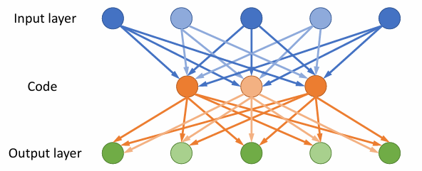
As shown above, Input Layer + Code is the Encoder, while Code + Output Layer is the Decoder.
Encoder transforms data into a more computationally friendly format, while Decoder trans into human-friendly.
不过事实上,Autoencoders最常见的用途是,通过学习正常的模式来检测异常:
- 训练时,只用正常数据
- encoder学习正常模式,decoder重建
- 重建误差越大,越可能是异常
当然了,此外还有一些其他的应用,比如图像去噪(医学影像)
Convolutional Layers
- N: input size
- F: filter size
- P: padding
- S: stride